The GAN objective, from practice to theory and back again

The GAN objective commonly used in practice

When I first learnt about GANs (generative adversarial networks)¹ I followed the “alternative” objective (which I will refer to as $G_{alt}$), which is the most common GAN objective found in the wild at the time of writing. You can see an example of it in DCGAN², which is available on GitHub.

$G_{alt}$ corresponds to the following update steps:

• Updating discriminator parameters: We want the discriminator to be good at telling generated images apart from real dataset samples. This can be thought of as a binary classification problem. Simply slap a sigmoid activation onto the end of the discriminator network and use binary cross entropy loss (nn.BCECriterion in Torch) with target 1 for “real” images and 0 for “fake” images.
• Updating generator parameters: We want the generator to be good at fooling the discriminator into thinking that generated images are real. This can be achieved by doing a forward pass through the discriminator with generated images, setting the BCE target to 1 (“real” images) and then calculating the gradient of the loss with respect to the image. The gradient effectively tells us how the generator can change its output to best fool the discriminator into thinking that it is a real image from the dataset. This gradient can then be backpropagated through the generator to update its parameters.

With the Power of Mathematics™ we can express the loss functions used in the above update steps.

Let

• $V(x;\omega)$ = discriminator (excluding final activation)
• $G(z;\theta)$ = generator
• $\sigma(v)$ = sigmoid activation function
• $\mathcal{L}_{BCE}(\hat{y}, y)=-y\log(\hat{y})-(1-y)\log(1-\hat{y})$ = binary cross entropy loss

Discriminator update, “real” examples $x\sim X_{data}$:

$$ \mathcal{L}_{real}(x) =\mathcal{L} _{BCE}(\sigma(V(x;\omega)), 1) =-\log(\sigma(V(x;\omega))) $$

Discriminator update, “fake” examples $x\sim G(Z;\theta)$:

$$ \mathcal{L}_{fake}(x) =\mathcal{L} _{BCE}(\sigma(V(x;\omega)), 0) =-\log(1-\sigma(V(x;\omega))) $$

Generator update:

$$ \mathcal{L}_{gen}(z) =\mathcal{L} _{BCE}(\sigma(V(G(z;\theta);\omega)), 1) =-\log(\sigma(V(G(z;\theta);\omega))) $$

A bit of theory

Imagine that $q(x)$ is the true probability distribution over all images, and that $p(x)$ is our approximation. As we train our GAN, the approximation $p(x)$ becomes closer to $q(x)$. There are multiple ways of measuring the distance of one probability distribution from another, and functions for doing so are called f-divergences. Prominent examples of f-divergences include KL divergence and JS divergence.

Somewhere in our practical formulation of the GAN objective we have implicitly specified a divergence to be minimised. This wouldn’t matter very much if our model had the capacity to model $q(x)$ perfectly, since the minimum would be achieved when $p(x)=q(x)$ regardless of which divergence is used. In reality this is not the case, and even after perfect training $p(x)$ will still be an approximation. The kicker is that the “best” approximation depends on the divergence used.

For example, consider a simplified case in one dimension where $q(x)$ is a bimodal distribution, but $p(x)$ only has the modelling capacity of a single Gaussian. Should $p(x)$ try to fit a single mode really well (mode-seeking), or should it attempt to cover both (mode-covering)? There is no “right answer” to this question, which is why multiple f-divergences exist and are useful.

Fig 1. Which is the better approximation? The answer depends on the f-divergence you are using!

Poole et al. ³ have worked backwards to find the f-divergence being minimised for $G_{alt}$. It turns out that the divergence is not a named or well-known function. The authors argue that the GAN divergence is on the mode-seeking end of the spectrum, which results in a tendency for the generator to produce less variety.

Generalising the GAN objective

It would be nice to specify whichever divergence we wanted when training a GAN. Fortunately for us, f-GAN⁴ describes a way to explicitly specify the f-divergence you want in the GAN objective.

Essentially the parts of the practical GAN objective specified earlier that imply the divergence are the sigmoid activation and the binary cross entropy loss. By replacing these parts with generic functions, we reach a more general formulation of the loss functions.

Discriminator loss

$$ \mathcal{L}_{real}(x) =-g _f(V(x;\omega)) $$

$$ \mathcal{L}_{fake}(x) =f^*(g _f(V(x;\omega))) $$

where $g_f(v)$ = an activation function tailored to the f-divergence, and $f^*(t)$ = the Fenchel conjugate of the f-divergence. A table of these functions can be found in the f-GAN paper, and they are relatively straightforward to implement as part of a custom criterion in Torch.

By setting $g_f(v) = \log(\sigma(v))$ and $f^*(t) = -\log(1 - e^t)$ we get the same discriminator loss functions as $G _{alt}$.

Generator loss

In the f-GAN paper, the generator loss is the same as $\mathcal{L}_{real}$:

$$ \mathcal{L}_{gen}(z) =-g _f(V(x;\omega)) $$

Pretty simple stuff here, really.

Poole et al. propose an extension which allows the generator and discriminator to be trained with different f-divergences. Roughly speaking this involves undoing the effects of the discriminator f-divergence to recover the density ratio $\frac{q(x)}{p(x)}$, and then applying the generator f-divergence $f_G$.

$$ \mathcal{L}_{gen}(z) =f_G((f’)^{-1}(g _f(V(x;\omega)))) $$

Field notes and thoughts

• Some generator f-divergences simply don’t train well. For instance, I was unable to successfully train a DCGAN variant using KL divergence for the generator. I think that the reason for this is that when you simplify the generator loss, it becomes $V(x;\omega) e^{V(x;\omega)}$. This means that if the discriminator learns to correctly recognise fake images, $V(x;\omega)$ will be a large-ish negative number and the generator loss will be vanishingly small thanks to the exponent. That is, the discriminator will effectively crush the generator and prevent it from learning. Analysing the loss curves confirms this, as the discriminator loss rapidly plummets to zero in a few epochs. This is not an issue reported by Poole et al., which might possibly be due to their discriminator architecture being somewhat crippled in comparison to DCGAN.
• I’m unsure of why it is a good idea to use different divergences for the discriminator and generator. Why not always use the same for both? I did find that doing this with reverse-KL caused the generator loss to spike quite severely, so perhaps it is a practical concern related to numerical precision?
• During implementation I noticed that JS divergence and GAN divergence are incredibly similar, with a only a few constants hanging around that make them different.

Here are some generated examples after training DCGAN on CIFAR-10 with different divergences, using the f-GAN generator loss.

f-divergence	Generated output
GAN divergence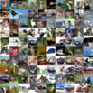
JS divergence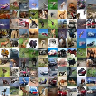
RKL divergence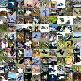

References

Generative Adversarial Networks. https://arxiv.org/abs/1406.2661 ↩︎
Unsupervised Representation Learning with Deep Convolutional Generative Adversarial Networks. https://arxiv.org/abs/1511.06434 ↩︎
Improved generator objectives for GANs. https://arxiv.org/abs/1612.02780 ↩︎
f-GAN: Training Generative Neural Samplers using Variational Divergence Minimization. https://arxiv.org/abs/1606.00709 ↩︎